Financial Data Forecasting Using R
To design and develop the best model for daily historical Apple stock prices (open, high, low, close and adjusted prices)
Supervisor: Professor Pan Guangming, Professor at Nanyang Technological Univeristy
Time: May, 2020
Github Repositoty: https://github.com/bozliu/Financial-Data-Forecasting
1 Objective
The objective of this article is to design and develop the best model for the financial data, the daily historical Apple stock prices (open, high, low, close and adjusted prices).
Note from Towards Data Science’s editors: While we allow independent authors to publish articles in accordance with our rules and guidelines, we do not endorse each author’s contribution. You should not rely on an author’s works without seeking professional advice. See our Reader Terms for details.
2 Plot Original Time Series Data
The adjusted prices for the daily prices of the Apple stock from February 1, 2002 to January 31, 2017 can be plotted, as shown in Figure 1. It can be observed that the mean value is not zero and the variance is very high. This indicates that the time series is non-stationary with varying mean and variance. The same collusion can also be drawn from its ACF plot, as shown in Figure 2 since it never dies down.


3 Log and One-Time Differencing Transformation
To stabilize the variance, the log return is taken, as shown in Figure 3. This time series plot shows that the mean is constant and nearly 0.

4 Augmented Dickey Fuller (ADF) Test
From the ADF test shown in Figure 4, it can be seen that the original data sequence is not stationary since its p value, 0.4882 is larger than 0.05, which rejects non-hypothesis. The data sequence after log return is stationary since its p value, 0.01 is smaller than 0.05, which rejects the hypothesis.

5 Autoregressive Conditional Heteroskedasticity (ARCH) Test
The time series data plot, Figure 3 shows that there may be ARCH effect in daily yield data. If there is ARCH effect, GARCH model can be fitted. Otherwise, GARCH model cannot be used to fit the data.
The result of ARCH test is shown in Figure 6. The original hypothesis of the test is that there is no arch effect. The test results show that the chi-square statistic value is 273.4, and the corresponding p value is almost 0. In order words, the original hypothesis is rejected at the significance level of 1%. Consequently, the log return of time series data has ARCH effect and therefore GARCH model can be fitted.

6 Exploratory Analysis
6.1 Distribution Shape
An overview of basic statistical values can be computed by the function basicStats. It reveals basic financial time series statistics, as shown in Figure 6. It can be seen that the mean is 0 and the distribution of log returns has heavy tail. The same conclusion can also be observed from QQ plot, as shown in Figure 7. Although there is a considerable derivation from the theoretical quantile of normal distribution, the series has a somewhat normal distribution with heavy tails at both ends as kurtosis is positive, equalling to 5.439298.


6.2 Auto-Correlation Function (ACF)
ACF plot of the log return of data, square of the log return of data and absolute of the log return of data respectively are shown in Figure 8. The ACF plots illustrate that since the log stock price returns are not correlated, the mean is constant for the time series. However, both the squared and the absolute stock price return values have high correlation. Thus, it could be concluded that the log returns process has a strong non-linear dependence.

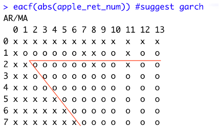
6.3 Extended Autocorrelation Function (EACF)
Using the absolute value of the log return of daily Apple stock price in EACF is better than square value of the log return of data due to the significant volatility of financial data. The EACF of the absolute value of the log return of data suggest GARCH (1,1) and GARCH (2,2), as shown in Figure 9 and Figure 10.

6.4 GARCH (1,1) Model
The summary of GARCH (1,1) and the p value of the generalized portmanteau tests with the squared standardized residuals from the fitted GARCH model are shown in Figure 12 and Figure 13 receptively. Although all the p value of generalized portmanteau tests with the squared standardized residuals are high than 5%, the p value of Jarque Bera Test is less than 5%. Hence, the normality assumption is rejected. Since the key model assumption is violated, a new model should be specified.


6.5 GARCH (2,2) Model
The summary of GARCH (2,2) and the p value of the generalized portmanteau tests with the squared standardized residuals from the fitted GARCH model are shown in Figure 14 and Figure 15 receptively. The p value of Jarque Bera Test is less than 5% and therefore the normality assumption is rejected. In addition, all the p value of generalized portmanteau tests with the squared standardized residuals are less than 5% suggesting that there is dependence of the squared residuals over time. Since the two key model assumption is violated, a new model should be specified.


6.6 Comparison between GARCH (1,1) and GARCH (2,2)
GARCH (1,1) is worthier to be further explored since it satisfies more key assumptions than GARCH (2,2).
7 Further Models Identification
7.1 GARCH (1,1) Model with Normal Distribution
The result of the fitted model, GARCH (1,1) with normal distribution is shown in Figure 16.
In terms of Ljung Box test for white noise behaviour in residuals, the residuals have p-values>0.05 and we fail to reject the null hypothesis, there is no evidence of autocorrelation in the residuals. Hence, we may conclude that the residuals behave as hite noise.
In terms of weighted Ljung-Box Test on standardized squared residuals and ARCH LM Test, the p-values>0.05 and we fail to reject the null hypothesis hence there is no evidence of serial correlation in squared residuals. This confirms that the residuals behave as a white noise process.
However, with regard to Adjusted Pearson Goodness-of-Fit Test, the normal distribution assumption is strongly rejected since p-values<0.05. Since the key model assumption is violated, a new model should be specified.

7.2 GARCH (1,1) Model with T-Distribution
The result of the fitted model, GARCH (1,1) with t-distribution is shown in Figure 17. In terms of the weighted Ljung-Box test on squared residuals, there is no evidence of serial correlation as the p-values>0.05 and hence the null hypothesis of serial correlation can be rejected, and we may conclude that the residuals behave as a white noise process. With regard to the goodness of fit test, since the p-values>0.05, the null hypothesis can’t be rejected and hence this model is a good fit. In other words, this model is adequate for this process.

7.3 GARCH (1,1) Model with Skewed T-Distribution
The result of the fitted model, GARCH (1,1) with skewed t-distribution is shown in Figure 18. Since the residuals have p-values>0.05 and we fail to reject the null hypothesis, there is no evidence of autocorrelation in the residuals. Hence, we may conclude that the residuals behave as hite noise. The standardized squared residuals and ARCH LM Tests shows the p-values>0.05 and we fail to reject the null hypothesis hence there is no evidence of serial correlation in squared residuals. This confirms that the residuals behave as a white noise process. With regard to the goodness of fit test, since the p-values>0.05, the null hypothesis cannot be rejected and hence this model is a good fit.

7.4 eGARCH (1,1) Model with T-Distribution
The result of the fitted model, eGARCH (1,1) with t-distribution is shown in Figure 19. In terms of Residual diagnostics, all the p-values for the Ljung Box Test of residuals are > 0.05, thus indicating that there is no evidence of serial correlation in the squared residuals and hence, they behave as white noise process. With regard to the test for goodness-of-fit, since all the p-values > 0.05, we cannot reject the null hypothesis, and hence we may conclude that the eGARCH model with the t-distribution is a good choice.

7.5 fGARCH (1,1) Model with T-Distribution
The result of the fitted model, fGARCH (1,1) with t-distribution is shown in Figure 20. In terms of residual diagnostics, all the p-values for the Ljung Box Test of residuals are > 0.05, thus indicating that there is no evidence of serial correlation in the squared residuals and hence, they behave as white noise process.
With regard to the test for goodness-of-fit, since all the p-values > 0.05, we cannot reject the null hypothesis, and hence we may conclude that the fGARCH model with the t-distribution is a good choice.

7.6 iGARCH (1,1) Model with Normal Distribution
The result of the fitted model, iGARCH (1,1) with normal distribution is shown in Figure 21. In terms of residual diagnostics, all the p-values for the Ljung Box Test of residuals are > 0.05, thus indicating that there is no evidence of serial correlation in the squared residuals and hence, they behave as white noise process. With regard to the test for goodness-of-fit, since all the p-values > 0.05, we cannot reject the null hypothesis, and hence we may conclude that the iGARCH model with the t-distribution is a good choice.

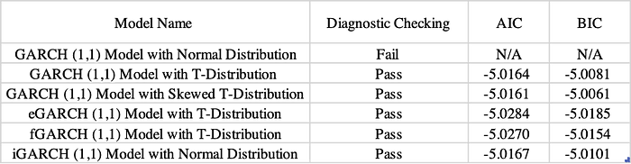
7.7 Model Selection
The AIC and BIC value of each possible model is show in the Table 1. It can be observed that the best model is eGARCH (1,1) model with t-distribution as the model has the lowest AIC value, -5.0284 and BIC value, -5.0185.
8 Forecasting
Different forecasting plots is shown in Figure 22. The sigma of the forecast, is the predicted conditional volatility at time t+h. Series represent the conditional mean at time t+h. The predicted mean is observed to be constant because the mean model on rt is constant. Predicted volatility converges to overall (unconditional) standard deviation of time series.

9 Conclusion
GARCH (2,2), GARCH(1,1) with normally distributed errors, GARCH(1,1) model with t-distribution, GARCH(1,1) model with skewed t-distribution, eGARCH(1,1) model with t-distribution, fGARCH(1,1) model with t-distribution, and iGARCH (1,1) model with normal distribution are applied to fit the data from the daily historical Apple stock prices(open, high, low, close and adjusted prices) from February 1, 2002 to January 31, 2017.
To sum up, the eGARCH (1,1) model with t-distribution is selected for the most appropriate model to fit and predict trend in the apple stock prices over the past 15 years.