Seasonal Data Forecasting Using R
To build a relative accurate model to predict the drug sales time series data
Supervisor: Professor Pan Guangming, Professor at Nanyang Technological Univeristy
Time: March, 2020
Github Repository: https://github.com/bozliu/Seasonal-Data-Forecasting
1 Objective
The objective of this article is to build a time series analysis model to predict the drug sales time series data.
2 Plot Original Time Series Data
The original data for monthly anti-diabetic drug sales in Australia from 1992 to 2008 can be plotted, as shown in Figure 1. There are a clear increasing trend and a strong seasonal pattern that increases in size as the level of the series increases.

3 Box-Cox Transformation
It can also be seen from Figure 1 that there is a small increase in the variance with the level, and therefore Box-Cox transformation can be applied to stabilise the variance. Lambda minimizes the coefficient of variation, and its optimal value can be found through BoxCox.lambda of the original data in R. The result of lambda is 0.1313326. Data after Box-Cox transformation is shown in Figure 2.

4 Seasonal Differencing
The data are strongly seasonal and obviously non-stationary, and therefore seasonal differencing will be used. As for the monthly data, frequency, and lag equal to 12. The seasonally differenced data are shown in Figure 3.

After seasonal differencing, the resulting series is fairly stationary according to the ACF (autocorrelation function) plot, as shown in Figure 4.

5 Unit Root Tests
Statistical tests can be applied to determine if data after seasonal differencing requires an order of differencing to improve stationary.
5.1 Augmented Dickey Fuller (ADF) Test
From the ADF test shown in Figure 5, it can be seen that the original data sequence is not stationary since its p value is larger than 0.05, which rejects non-hypothesis. The data sequence after seasoning difference is stationary since its p value is smaller than 0.05, which rejects the hypothesis.

5.2 Kwiatkowski-Phillips-Schmidt-Shin (KPSS) Test
From KPSS test shown in Figure 6, it can also be seen that the original data sequence is not stationary since its p value is smaller than 0.05, which rejects the hypothesis. The data sequence after seasoning difference is level stationary since its p value is larger than 0.05, which rejects the non-hypothesis.

Hence, data after seasonal differencing is stationary, and there is no need to apply the order differencing.
6 Fitting in Different Models
Total observations of original data can be separated into training data with 80 percent observations and testing data with 20 percent observations.
6.1 Linear regression model with seasonal and trend features
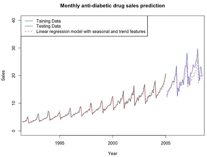
Figure 7 reveals the comparison between the training data and fitted data for the linear regression model, between the testing data and prediction value based on the model.
6.2 Holt-Winters model with additive seasonal components
Figure 8 shows the comparison between the training data and fitted data for the holt-winters model with additive seasonal components, between the testing data and prediction value based on the model.

6.3 Holt-Winters model with multiplicative seasonal components

Figure 9 demonstrates the comparison between the training data and fitted data for the holt-winters model with multiplicative seasonal components, between the testing data and prediction value based on the model.
6.4 Seasonal autoregressive integrated moving average model
Auto ARIMA function is applied to find the most appropriate p, q, P, and Q. When models are compared using AIC values, it is important that all models have the same orders of differencing. Based on previous exploratory analysis, the order differencing, d sets to 0 and the seasonal differencing, D sets to 1.
The maximum value of p, q, P and Q are set to 5, and therefore Auto ARIMA function can look for each value from 0 to 5 and find out the most appropriate model with minimum AIC value. According to the result, as shown in Figure 10, p=3, q=0, P=0, Q=2 and AIC= -451.98. In addition, the model is verified to be adequate by diagnostic checking, as shown in Figure 11.


Figure 12 demonstrates the comparison between the training data and fitted data for the seasonal autoregressive integrated moving average model, between the testing data and prediction value based on the model.

7 Evaluation
It can be seen from Table 1 that the seasonal autoregressive integrated moving average model performs the best in the testing data when the forecasting horizon is 62 months measured by RMSE (Root Mean Squared Error), MAE (Mean Absolute Error) and Theil’s U (Uncertainty coefficient). However, when looking at the other error metric, MAPE (Mean Absolute Percentage Error), the Holt-Winters model with multiplicative seasonal components is actually performing better than the ARIMA model. These error metrics are computed from the testing set, representing the observations on the black line in the plots. The observations on colourful dashed lines are the future forecasts of sales comparing with the testing set, representing the actual observations on the blue line in the plots.

8 Conclusion
Linear regression model with seasonal and trend features, Holt-Winters model with additive seasonal components, Holt-Winters model with multiplicative seasonal components, and Seasonal autoregressive integrated moving average model are applied to fit the data or monthly anti-diabetic drug sales in Australia from 1992 to 2008.
To sum up, the Seasonal autoregressive integrated moving average model, ARIMA(3,0,0) (0,1,2) [12] is selected for the most appropriate model to predict drug sales due to its smallest AIC value, RMSE value, MAE value and Theil’s U value among all the models.