Joint Approaches to Optimize End-To-End System for Robust Far-Field Wake-Up Keyword Detection
Demo
The demo is implemented to classify the 10 keywords “Yes”, “No”, “Up”, “Down”, “Left”, “Right”, “On”, “Off”, “Stop”, “Go” on Python. It can detect whether there are keywords in the speech in real time via the local device microphone. If there is a keyword, it will be highlighted in the pie chart, as shown in Figure 17. Otherwise, it would be treated as unknown.

Abstract
Wake-up word detection is also called, keyword spotting (KWS). It is an essential component to trigger the user voice on smart devices. In other to obtain good user experience, it needs real-time interaction and high accuracy. Neural networks have recently become a popular approach for keyword spotting, as they are superior to conventional voice processing algorithms. In this thesis, some typical popular networks are trained such as VGG, Deep Residual Network (ResNet), WideResNet (WRN), Densely Connected Convolutional Network (DenseNet), Dual Path Network (DPN) and Multi-head attention Based network in the objective of comparison in accuracy and storage. In addition, a novel loss function is proposed and implemented on the multi-head attention neural network. When comparing it against other neural network architectures, it achieves an accuracy of 98.2%, which outperforms the Start of Art Result in [1].
1 Contribution
(a) To transfer popular neural networks in image classification and natural language processing from the literature [2–7] to KWS field on Google speech commands dataset [8] and compare them in terms of accuracy and model parameters.
(b) To propose a novel loss function inspired by triplet loss used in face recognition [9] and implement it on the end-to-end multi-head attention model. This model outperforms the state-of-the-art performance in accuracy and relatively small model size.
(c) Discussion about how different model topology improves accuracy and makes the keyword spotting models explainable.
(d) To implement a demo to locally detect the keywords in real-time.
2 Feature Extraction
Speech signals can be digitally interpreted as a number sequence with the same number of items per second as the specimen rate. This representation, however, does not contain audio detection detail. To address this challenge, the extraction of features is often called voice parameterisation, using spectral features of an input audio signal to enable speech decoding. Fast Fourier transform (FFT) on a narrow audio window allows you to translate the raw audio to the frequency dominate. Whilst at any frequency band in the audio window the FFT contains energy information, it doesn’t stress the band that is critical for human hearing, which is below roughly 1000 Hz. Davis etal.[10] proposed a cepstral coefficient Mel frequency to imitate the behaviour of the human ear in order to solve this challenge. The main steps involved in computing MFCC features are shown in Figure 1.

3 Standard End to End KWS System
The standard end to end model architecture of KWS consists of a feature extractor and a neural network based classifier, as shown in Figure 2. An input audio signal is fed into a speech feature extractor. Function extraction through Log-Mel bank energy filters (LFBE) or mel frequency cepstral coefficients (MFCCs) involves the translation of the spoken time domain signal into a collection of spectral frequency-domains coefficients that allow input signal dimension compression. The extracted features are classified by a neural network which produces the probabilities of the output classes. The model could be trained by using a loss function with an optimizer, such as the cross-entropy loss function with Adam optimizer. Overall, the definition of end-to-end model can directly outputs keyword detection with no complicated searching involved and no alignments needed beforehand to train the model.

4 Multi-Head Attention Based Network Architecture
Most of the current state-of-the-art keyword spotting architectures are present in the work of Rybakov et al. [1], with the best model to date being the Bidirectional GRU-based Multiheaded attention RNN. It takes a spectrum in Mel scale and complements it with a series of 2D convolutions. The Audio Data is then used with two two-way long-term relationship to record two-way GRU layers. The function in the middle of the bidirectional GRU output series is projected with a dense layer and is used as a multi-head (4-head) query vector. At present, the GRU layer output is sampled, projected with a thick layer to distinguish which portion of the audio is more significant and is used as question vectors. The weighted average bidirectional GRU performance (by attention) is ultimately processed by a series of completely connected classification layers.

5 Loss Function
5.1 Cross Entropy Loss
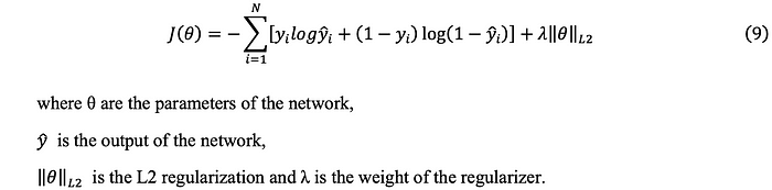
With regard to multi-class classification problem, the network is generally trained using standard multi-class cross entropy loss with L2 regularization. Its objective function is shown in Equation (9).
5.2 Triplet Loss
Triplet loss is a loss function of deep learning, which is mainly used to train samples with small differences, such as faces. Also, triplet loss is often used in embedding tasks, such as text and image embedding. The loss function of triplet loss is shown in Equation (10).
The input is a triple, including anchor, positive and negative. By optimizing the distance between anchor and positive is less than that between anchor and negative, the similarity between samples is calculated. The final optimization goal is to shorten the distance between a and p, and to extend the distance between a and n.

5.3 Proposed Novel Loss
Inspired by triplet loss, the loss feature is designed to minimize the sample distance from one keyword and increase the sample distance from various keywords. In the updated KWS model, the SoftMax layer is omitted, and the output of the penultimate layer is a fixed-dimensional vector that maps the function of the input keyword into a fixed-dimensional space instead of direct prediction effects with a soft max layer. This fixed-dimension vector can be compared with the template keyword feature representation obtained by Equation (11).

The similarity matrix between sample’s output vector and the centroids can be computed by the cosine similarity value. Assume S_c:keyword as the similarity matrix between the sample output vector and the centre vector of the keyword and S_c:nonkeywords as the similarity matrix between sample’s output vector and the centroids of the non-keywords. As for , the bigger the value of the cosine, the closer the sample is to the keyword. The loss function can be calculated in Equation (12).

6 Experiments
6.1 Speech Command Dataset
Version 1 (V1) of the Command Speech Dataset [8] includes 30 commands made up of 64,727 utterances spoken by 1881 speakers, respectively. A single utterance, captured in wave format at 16 kHz, was used for each audio length for one second. In addition, the dataset provides six types of noises such as running tap, doing dishes, white noise, pink noise, etc. A few noises are recorded in real time while others were computer-generated. Table 1 presents the descriptions of orders and noises. These data sets were collected and primarily supported by European citizens inside a managed climate.

6.2 Data Augmentation
6.2.1 Time shifting
Time shifts are added to each study with a 50 per cent possibility. The increased collections are up to 20 per cent of the initial duration moved forward or backward in time. Perhaps, this may lead to a partial decrease in the utterance of the sample, but the chances are insignificant. This strategy to increase the model is designed to help the interpretation of words more time-invariant, since they can appear anywhere in model learning.
6.2.2 Amplitude Scaling
The amplitude of samples is 50% probability randomly scaled with the range from -50db to 50db.
6.2.3 Mixing with Noise
Mixing the samples with noise is introduced at a probability of 50 percent. There is noise produced in the same way as silence is generated when up to two samples are scaled and added together from the background audio of the dataset. The initial input, which was scaled from 75 and 125% of the original amplitude, was then applied to this noise. The addition of noise can help the model differentiate better from data pertinent information.
6.3 Training Details
The input to the model is the raw WAV data with original sampling rate of ∼16 kHz. In the stage of feature extraction, Mel-scale spectrogram is computed using 80-band Mel scale, 1024 discrete Fourier transform points and hop size of 128 points (∼8 s).
With a batch size of 512, the models are trained in PyTorch for 50 iterations with the Adam optimizer and initial learning rate of 0.0001. L2 regularization is set to 0.0001. The ReduceLROnPlateau in PyTorch is applied as the learning rate scheduler to adjust the learning rate when the loss of the verification set no longer decreases. The trained models are evaluated based on the classification accuracy on the test set.
7 Experimental Results
7.1 Evaluation of Different KWS Models
The popular neural network architectures, VGG, ResNet, WideResNet, denseNet, DPN and multi-head attention, are implemented. The result is shown in Table 2.

In VGG, deeper network achieved better performance whereas in ResNet, simply increasing the depth of the neural network obtained worse performance, brought difficulties to the training and caused non-convergence problems. In other words, despite the constraints of numerical computing and memory, networks with multiple filters and less layers achieved greater accuracy than networks with multiple layers and fewer filters. The first layer detects the characteristic patterns of input voice features and each following convolutional layer detects patterns in the previous layer patterns, introducing an abstraction degree. Therefore, an explanation of the effects of the grid quest may be that if the network has enough abstraction levels (layers), the number of different patterns required for the spoken contents (filter numbers) at each abstraction level will be very small. Even if the network with many layers, the network does not learn much useful information. On the other hand, the constrain of large filter size is to cause much trainable parameters. Despite VGG achieved higher accuracy than ResNet, it also consumes more computing resources and uses more parameters.
The best KWS models is multi-head attention-based network. It achieves a balance between memory and operations while still achieving good accuracy.
7.2 Evaluation on the Proposed Loss Function
These models have been updated to identify the user-defined keywords by extracting the layer SoftMax and compare the performance vector of the keyword to each keyword’s prototype.
The proposed loss function is applied on multi-head attention model as it shows relatively good performance. Table 3 shows the comparison of recognition accuracy between using cross-entropy and the proposed loss function. From Table 8, it can be seen that with the new loss function, the recognition of KWS system increases significantly by around 0.6% for the models.

8 Possible Improvements
8.1 Evaluating Models on FRR and FAR Matric
Although our model is close to 100% in accuracy, we can try to improve my model in another indicator. It is important to keep the count of false alarms as low as possible for devices that are still in use. In this case, FRR and FAR can be used to replace accuracy as the prioritized evaluation metric. The ratio of negative to positive samples in training, i.e. utilizing more ‘unknown’ and ‘silence’ samples, could become an optional tool for reducing FPR and increasing the true negative rate. In other machine learning detection tasks this has been shown to be an efficient approach. The FPR may also be reduced by creating a failure feature for the optimizer during training that penalizes errors that trigger false alarms rather than missing errors.
8.2 Reducing Model Size by Teacher-Student (T/S) Learning
In [58], a typical DNN model was proposed to compact the teacher-pupil (T/S) learning. Learning is the soft mark created by the instructor paradigm as a goal of student learning for a student classification instruction. The idea of “T/S learning” has been generalized to “the concept of information distillation”[59] by combining cross-entropy classification with the traditional cross-entropy classification workout using soft labeling and the single hot vector as the objective. As the regularization concept for the normal cross-entropy classification instruction, the soft objective for information distillation.
The constructed structures are generally an ensemble of gigantic models with many deep models. Unable to deploy such a device in real-time. In this case, learning or the distillation of information offers a good way to achieve a compact model with strong modelling capacity. T/S Compression has been a most recent achievement in producing a CTC model [60] with almost the same KWS, but with just a 1/27 footprint of a massive KWS CTC model.
9 Conclusion
Various Neural Network Architectures in including VGG, Deep Residual Network (ResNet), WideResNet (WRN), Densely Connected Convolutional Network (DenseNet), Dual Path Network (DPN) and Multi-head attention Based network were trained and compared. In addition, inspired by Triplet loss, a novel loss function is proposed and implemented on Multi-head Attention Based Network. The experimental results show that the Multi-head Attention Based Network achieved the best accuracy, 97.6% and with the proposed loss function, the accuracy is further improved to 98.2%, which matches or exceeds the state-of-the-art result.
Bibliography
[1] Rybakov, O., Kononenko, N., Subrahmanya, N., Visontai, M., & Laurenzo, S. (2020). Streaming keyword spotting on mobile devices. arXiv preprint arXiv:2005.06720.
[2] Simonyan, K., & Zisserman, A. (2014). Very deep convolutional networks for large-scale image recognition. arXiv preprint arXiv:1409.1556.
[3] He, K., Zhang, X., Ren, S., & Sun, J. (2016). Deep residual learning for image recognition. In Proceedings of the IEEE conference on computer vision and pattern recognition (pp. 770–778).
[4] Zagoruyko, S., & Komodakis, N. (2016). Wide residual networks. arXiv preprint arXiv:1605.07146.
[5] Huang, G., Liu, Z., Van Der Maaten, L., & Weinberger, K. Q. (2017). Densely connected convolutional networks. In Proceedings of the IEEE conference on computer vision and pattern recognition (pp. 4700–4708).
[6] Chen, Y., Li, J., Xiao, H., Jin, X., Yan, S., & Feng, J. (2017). Dual path networks. arXiv preprint arXiv:1707.01629.
[7] Vaswani, A., Shazeer, N., Parmar, N., Uszkoreit, J., Jones, L., Gomez, A. N., … & Polosukhin, I. (2017). Attention is all you need. arXiv preprint arXiv:1706.03762.
[8] Warden, P. (2018). Speech commands: A dataset for limited-vocabulary speech recognition. arXiv preprint arXiv:1804.03209.
[9] Schroff, F., Kalenichenko, D., & Philbin, J. (2015). Facenet: A unified embedding for face recognition and clustering. In Proceedings of the IEEE conference on computer vision and pattern recognition (pp. 815–823).
[10] Davis, S.; Mermelstein, P. Comparison of parametric representations for monosyllabic word recognition in continuously spoken sentences. IEEE Trans. Acoust. Speech Signal Process. 1980, 28, 357–366.